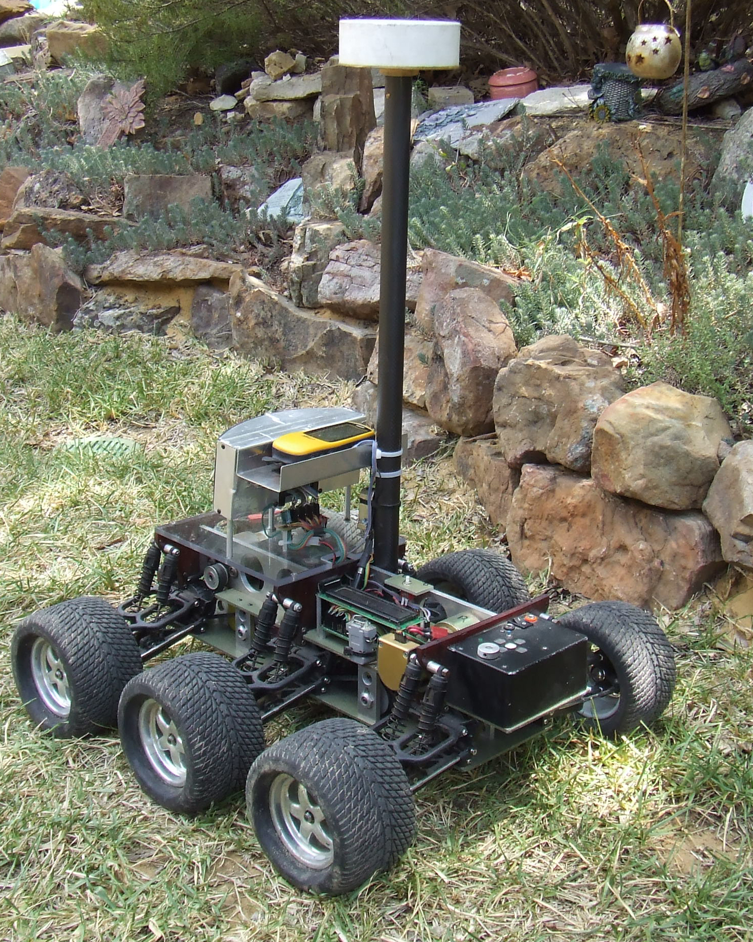
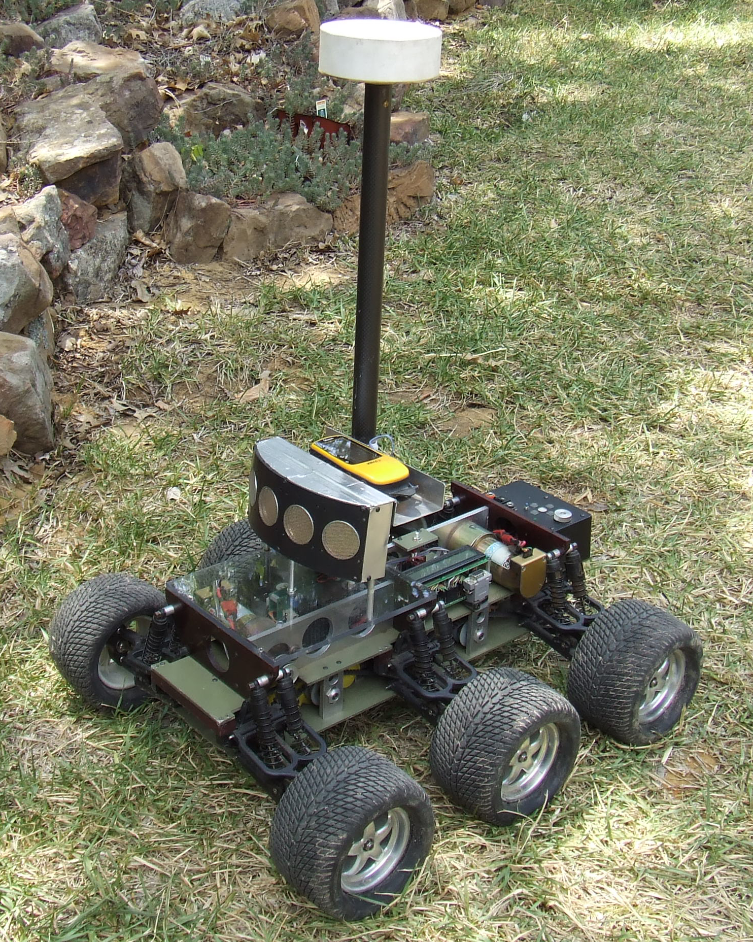
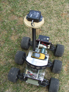
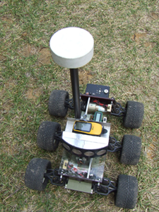
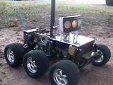
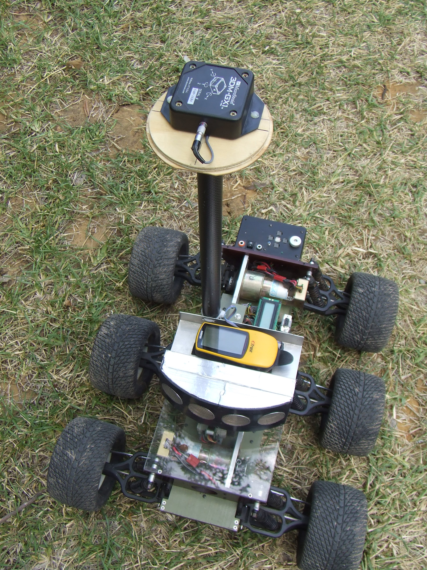
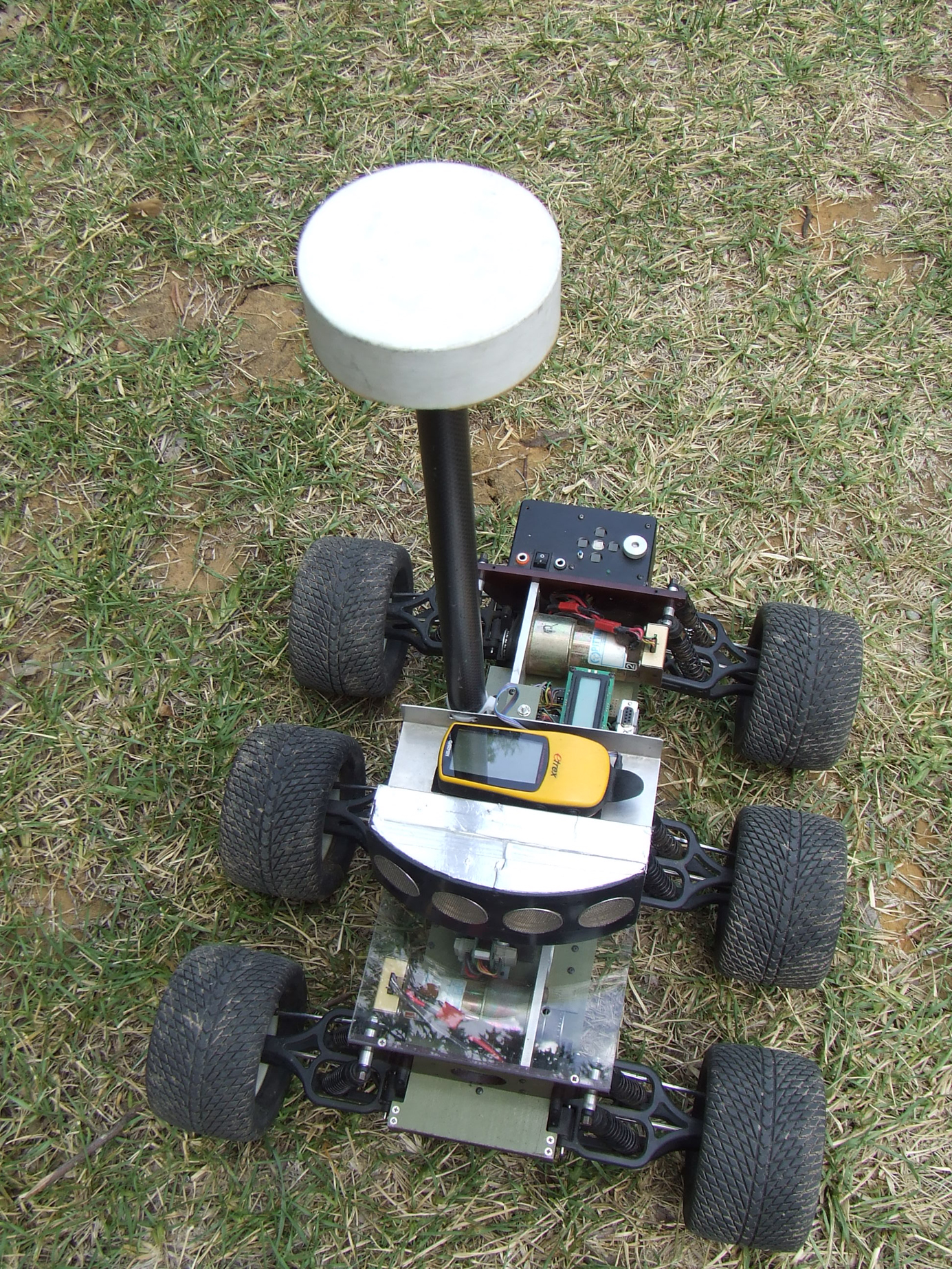
Two views of the jBot autonomous robot.
(click on images for higher resolution)

Table of Contents

1. Introduction
2. Odometry
3. Odometry Calibration and Error Analysis
4. Eliminating Accumulated Odometry Errors in Heading
5. The Microstrain 3DM-GX1
6. jBot's 3DM-GX1 Implementation
7. Integrating the 3DM-GX1 IMU with jBot's odometry
8. jBot's IMU-corrected Odometry performance
9. Other conditions measured by the IMU
10. Conclusions

I. Introduction

Howdy

The following is a description of the integration of a commercial Inertial Measurement Unit with the navigation algorithms of the jBot autonomous off-road robot. This allows the robot to navigate unstructured outdoor environments, without a GPS or other external reference, with an accuracy on the order of about .5% of the distance traveled. That is, a journey of 1000 feet has a location error on the order of 5 feet upon arrival at the destination.

For more information on jBot's navigation abilities see:

http://www.geology.smu.edu/~dpa-www/robo/jbot/

and especially the videos of the robot navigating through the Texas woods and the Colorado Rockies.

II. Odometry

The classical technique for a wheeled robot to calculate its position is to track its location through a series of measurements of the rotations of the robots' wheels, a method often termed "odometry." The roboticists' standard reference for location calculations is the seminal theses by Johannes Borenstein titled "Where Am I?" which covers the topic in detail, with equations, proofs, and samples. Every robot builder should have this book:

http://www-personal.engin.umich.edu/~johannb/position.htm

A. Encoders

Odometry requires a method for accurately counting the rotation of the robot wheels. A standard method for doing this is to instrument the wheels with optical shaft encoders. For my LegoBot, SR04 robot, and nBot balancing robot, the encoders are handmade from Hamamatzu sensors reading paper encoder disks created with a laser printer. Here's a link for those robots:

http://www.geology.smu.edu/~dpa-www/myrobots.html

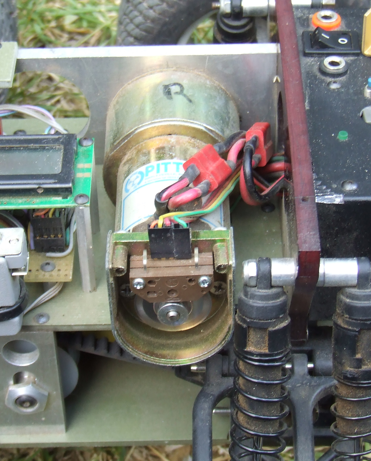
and a link describing how to add home-brew encoders to a Pittman gear-head motor, like those used on nBot:

http://www.geology.smu.edu/~dpa-www/robo/Encoder/pitt_html/encoders.html

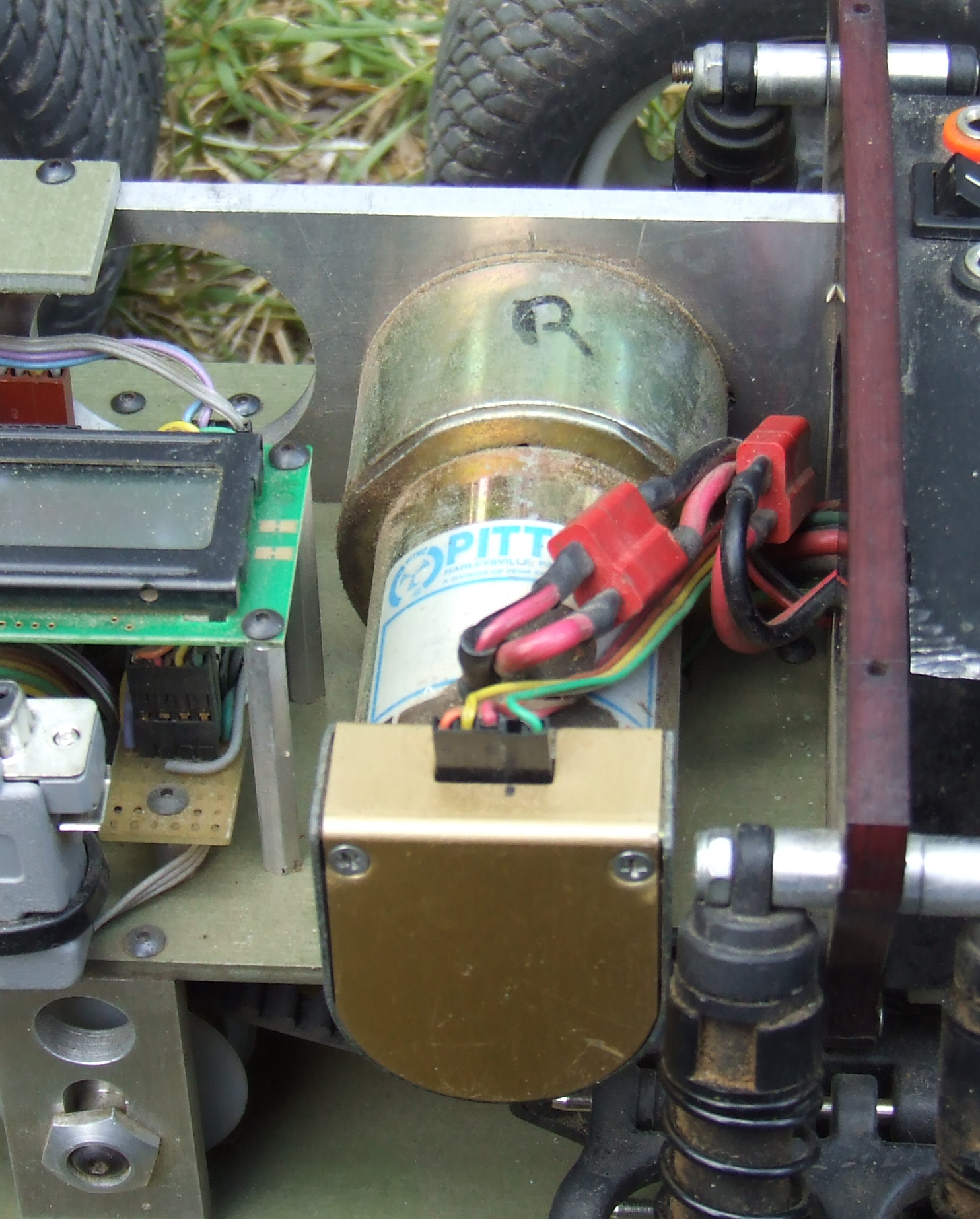
The encoders for LegoBot are attached to the drive axles, but for SR04 and nBot they are attached directly to the motors themselves. jBot uses two Pittman gear-head motors with integrated optical encoders. Here are two images of the right gear-head motor with its integrated encoder. The second image is of the encoder with it's protective cover removed:

In all four robots, the encoders are used to generate interrupts on the main controlling microprocessor, which maintains 32-bit counters of the encoder ticks. LegoBot, SR04, and nBot generate counts with a resolution on the order of 1 count per 1/16th of an inch of travel. The encoders on jBot produce 2000 counts per revolution of the motor shaft, about 4323 counts per inch of wheel travel. This is way more than are needed, but better too many than too few.

On nBot and jBot, the encoders generate quadrature signals which allow the robot to determine both velocity and direction of the wheels. The other two robots have only single channel encoders for measuring velocity, and deduce the wheel direction from the sign of the last motor command sent to the wheels, which seems to work just as well. A more detailed account of the software used on SR04 is available from:

http://www.geology.smu.edu/dpa-www/robots/doc/odometry.txt

and for jbot:

http://www.geology.smu.edu/dpa-www/robo/subsumption/

B. Math

The simplest method of location calculation is for a differentially steered robot with a pair of drive wheels and a castering tail or nose wheel. Other geometries such as traditional rear-wheel-drive with front-wheel Ackerman steering can also work but may require more complex calculations, depending on how the vehicle is instrumented.

For the differentially steered robot, the location is constantly updated using the following formula. The distance the robot has traveled since the last position calculation, and the current heading of the robot, are calculated first:

(1)	distance = (left_encoder + right_encoder) / 2.0
(2)	theta = (left_encoder - right_encoder) / WHEEL_BASE;

where WHEEL_BASE is the distance between the two differential drive wheels.

Note the convention is (left-right) rather than what you may remember from trig class. For navigation purposes it is useful to have a system that returns a 0 for straight ahead, a positive number for clockwise rotations, and a negative number for counter-clockwise rotations.

With these two quantities, a bit of trig can give the robot's position in two dimensional Cartesian space as follows:

(3)	X_position = distance * sin(theta);
(4)	Y_position = distance * cos(theta);

You can multiply theta * (180.0/PI) to get the heading in degrees.

The robot's odometry function then tracks the robot's position continuously by accumulating the changes in X,Y, and theta 20 times per second, and maintains these three values: X_position, Y_position, and theta. These values create a coordinate system in which X represents lateral motion with positive numbers to the right and negative numbers to the left, Y represents horizontal motions with positive numbers forward and negative numbers back-wards, and theta represents rotations in radians with 0 straight ahead, positive rotations to the right, and negative rotations to the left.

The technique by which these values are used to steer the robot toward an assigned target position is beyond the scope of this article. (However, see the odometry.txt and subsumption files referenced above).

C. Sample Odometry Implementation

The SR04 robot is controlled by a Motorola HC11 8bit microprocessor. The encoder interrupts maintain the 32 bit counters "left_distance" and "right_distance." The following "C" code fragment is used by SR04 to calculate its location in inches from the origin 0,0 with heading 0, where it was last reset, using wheel odometry:

/* ----------------------------------------------------------------------- */

#define WHEEL_BASE 9.73
#define LEFT_CLICKS_PER_INCH 79.52
#define RIGHT_CLICKS_PER_INCH 79.48

/* ----------------------------------------------------------------------- */
/* odometer maintains these global variables: */

float theta;                    /* bot heading */
float X_pos;                    /* bot X position in inches */
float Y_pos;                    /* bot Y position in inches */

/* ----------------------------------------------------------------------- */


void odometers()
{
	int lsamp, rsamp, L_ticks, R_ticks, last_left, last_right;
	float left_inches, right_inches, inches;

        while (1) {

                /* sample the left and right encoder counts as close together */
		/* in time as possible */
                lsamp = left_distance;
                rsamp = right_distance; 

		/* determine how many ticks since our last sampling? */
                L_ticks = lsamp - last_left; 	
                R_ticks = rsamp - last_right;

		/* and update last sampling for next time */
                last_left = lsamp; 
                last_right = rsamp; 

		/* convert longs to floats and ticks to inches */
                left_inches = (float)L_ticks/LEFT_CLICKS_PER_INCH;
                right_inches = (float)R_ticks/RIGHT_CLICKS_PER_INCH;

		/* calculate distance we have traveled since last sampling */
                inches = (left_inches + right_inches) / 2.0;
	
		/* accumulate total rotation around our center */
                theta += (left_inches - right_inches) / WHEEL_BASE;

		/* and clip the rotation to plus or minus 360 degrees */
                theta -= (float)((int)(theta/TWOPI))*TWOPI;

		/* now calculate and accumulate our position in inches */
                Y_pos += inches * cos(theta); 
                X_pos += inches * sin(theta); 

		/* and suspend ourself in the multi-tasking queue for 50 ms */
		/* giving other tasks a chance to run */
                msleep(50);
        }
}

This task is one of several that are run by the robot's multitasking kernel. It runs 20 times per second and maintains the robot's location on a 1 inch grid. It maintains the variables X_pos, Y_pos, and theta, the heading of the robot in radians, relative to its origin at 0,0 heading 0, the location and orientation of the robot when last reset.

III. Odometry Calibration and Error Analysis

A. Calibration

Standard odometry as described for the SR04 robot requires calibration of the following constants: WHEEL_BASE, LEFT_CLICKS_PER_INCH, and RIGHT_CLICKS_PER_INCH. The calibration technique, Borenstein's UMBmark, is described in detail in the document:

http://www-personal.engin.umich.edu/~johannb/Papers/umbmark.pdf

1. The encoders are first calibrated by driving the robot in a straight line for a fixed distance and recording the total number of encoder counts for each wheel. The average of these counts is divided by the total distance traveled to get a starting value for encoder clicks_per_inch:



(5)	clicks_per_inch = ((left_counts + right_counts)/2) / total_inches_traveled


It is convenient to use the 1 foot square tiles found in most large institutional building hallways as a sort of graph paper for making this measurement. One hundred tiles is a good approximation of 1200 inches. Borenstein suggests that ten tiles are sufficient.


2. Calibration of the WHEEL_BASE and differences between the two wheels are then measured by having the robot drive a series of large squares, clockwise and counter-clockwise, while recording the errors in X_position and Y_position as compared to the original starting location. See the UMBmark paper for additional details, including a method for autonomous robot self-calibration.



3. Using Borenstein's UMBmark, the SR04 robot achieves an average accuracy on a smooth surface of about 6 inches on a 10 foot square, or about 1.25% of distance traveled.

Here is a 7.6 Meg mpeg video of the SR04 robot running clockwise around a 10 foot square consisting of four waypoint coordinates, in inches: (0,120) (120,120) (120,0) (0,0). The starting location (0,0) is marked on the floor with masking tape in order to better visualize the error on the robot's return.

There are two additional challenges on this square which the robot must avoid using it's SONAR, so it is not a pure calibration run. One is an architectural barrier between the second and third waypoints, and the other is a moving foot -- my own -- in front of the last waypoint, illustrating the odometry-driven navigation's ability to deal with unplanned static and dynamic obstacles while maintaining its nominal position accuracy.

http://www.geology.smu.edu/~dpa-www/robots/mpeg/sr04_sq_001x.mp4

B. Error analysis

The calculated position of the robot drifts over time as the errors in odometry accumulate, mostly from wheel slippage and uneven surfaces. Observations of the position error of the SR04 robot in carefully controlled environments reveal that the largest errors are those that accumulate in the theta value: the heading of the robot.

For example, suppose both wheels on the robot slip once by 1/2 inch. In terms of the distance calculations, this is not very significant, as the robot will arrive 1/2" short of its destination. On a trip of 100 feet, that is an error of only about .04 percent.

But for theta calculations, an error of 1/2" between the two wheels is much more serious, resulting in large errors in both X and Y position.

For a robot with a 10 inch WHEEL_BASE, a single slip of 1/2 inch by one of the wheels results in a heading error of .05 radians, about 3 degrees:

(6)	heading error 	= (left - right)/WHEEL_BASE
			= .5/10 
			= .05 radians * (180/PI) = 2.8 degrees

So for a robot that is driving in a straight line forward for 100 feet, with no error in heading (0 radians), it will arrive at location:

(7)	X = 100' * sin(0) = 0'
	Y = 100' * cos(0) = 100'

But for a robot driving in a straight line forward for 100 feet with an error in heading of only .05 radians, corresponding to a single 1/2 inch slippage between the two wheels, the robot will arrive at location:

(8)	X' = 100' * sin(.05) =  4.88 feet
	Y' = 100' * cos(.05) = 99.88 feet

and the X location will be off by almost 5 feet.

       X,Y 
        |      X',Y'
        |      /
        |     /
        |    /
        |   /
        |  /
        | /
        |/
       0,0

   (not to scale)

Thus small errors in theta produce large errors in X and Y. A visual example of the error created by a single wheel slip at the beginning of a run as measured by Borenstein's UMBmark might look like this:

       B--------------------C
        |     B /\         |
        |      /  \        |
        |     /    \       |
        |    /      \      |
        |   /        \     |
        |  /          \    |
        | /            \   |
        |/             /C  |
       A-\------------/-----D
          \          /
           \        /
            \      /
             \    /
              \  /
               \/D


          (not to scale)

The length of the sides of the squares are identical, as determined by the distance traveled, but the orientation of the squares are substantially different.

Obviously this might not be accurate enough to keep a robot within a confined space, such as a room or robot contest course, and the robot might even attempt to reach coordinates that are within walls or other unreachable locations. For short runs, as is typical of most robot contests, this is not a problem. But for extended runs, the accumulated errors become significant.

C. Error correction

From the above analysis it can be seen that the most important error in the robot's position calculation is the error in heading, the theta calculation.

The SR04 robot control algorithm used for various experimental robot contests takes advantage of the fact that robot contest courses invariably have parallel and horizontal walls.

The robot periodically scans the walls using its two forward-looking SONAR units to "square" itself to the walls, thus correcting drift in theta. Once so aligned, it measures the distance to a pair of walls at right angles to correct any errors in X,Y.

In the following 15 Meg mpeg movie, the SR04 robot is running the can collecting task for the Dallas Personal Robotics Group "CanCan" contest. After locating and fetching each can, the robot returns the can to the starting place. It then squares itself to the contest walls and measures their distance, using it's stereo SONAR, to correct drift in theta. The DPRG's Kipton Moravec provides commentary on the video.

http://www.geology.smu.edu/~dpa-www/robots/mpeg/cancan.mp4

A more sophisticated technique might keep a running measurement of the wall's location to prevent the drift in theta from accumulating in the first place, and thus obviate the need for such periodic recalibration.

As a general case I have found that the robot's position calculation will not drift significantly if errors in heading can be eliminated.

That seems worth restating as a first-order maxim for experimental robotics odometry:

(9)	IF 	ACCUMULATED ERRORS IN HEADING CAN BE ELIMINATED 
	THEN 	ACCUMULATED ERRORS IN DISTANCE CAN BE SAFELY IGNORED.

For a more detailed analysis of why this is so, see the appendix to Borenstein's UMBmark paper.

IV. Eliminating Accumulated Odometry Errors in Heading

The jBot robot is designed to operate in unstructured environments where it cannot depend on handy orthogonal walls for realignment, as does the SR04 robot. And although jBot has an on-board GPS unit, the availability of GPS signals cannot be depended on in all circumstances. (But see the navman Jupiter 12 Dead Reckoning system for a nifty possible work-around at www.navman.com).

A. Magnetic Compass

A number of robot builders have worked with magnetic compasses as a method for correcting heading errors. For example see:

http://www.seattlerobotics.org/encoder/200211/Compass.htm

which describes experiments with the Vector and Dinsmore electronic compasses. This approach is promising but suffers from two drawbacks for navigation purposes.

1. First, the compass is subject to local magnetic anomalies, which can cause the heading to swing by as much as 90 degrees as the robot passes large iron objects like cars or even the re-bar embedded in concrete.


2. Second, because the Earth's magnetic lines of flux "dip" in declination, the compass must remain level for the readings to be accurate. Some electronic compasses employ a 2-axis gimbal in an attempt to keep the compass level, but these are problematic in the rough off-road environments in which jBot is designed to operate.

B. Rate Gyro

An alternate method for maintaining an accurate heading for odometry calculations is the use of a rate gyro to hold the robot on course. This works very well for medium length robot runs, as Larry Barello (www.barello.net) has demonstrated with his group's FIRST competition robots.

However the heading calculated by integrating the output of a rate gyro is itself subject to drift over time, the very problem we are attempting to solve, so it is less useful for a robot, such as jBot, designed to cover kilometers rather than meters. For a more detailed approach to combining a rate gyro with odometry, see Borenstein's "Gyrodometry" paper:

http://www-personal.engin.umich.edu/~johannb/Papers/paper63.pdf

C. Gyro-corrected Magnetic Compass

Combining a magnetic compass and a rate gyro allows the strengths of each sensor to compensate for the weakness of the other. In this case, the gyro provides for accurate high frequency, moment-by-moment measurement of the robot's heading while ignoring local magnetic anomalies, while the compass provides a long-term North reference to correct for the drift of the the integrated gyro rate. For example see:

http://www.seattlerobotics.org/encoder/200311/brown/building_a_directional_gyro.html

which describes a home-brew system consisting of an ADXL rate gyro and a Devantech compass.

A more robust approach for combining the two sensors is the use of a Kalman filter or Weiner filter to characterize and compensate for the errors of each, the discussion of which is beyond the scope of this paper. For a good starting point see the paper on complementary filters at:

http://geology.heroy.smu.edu/~dpa-www/robo/balance/inertial.pdf

which describes an applicable technique for combining two devices as a tilt sensor.

Borenstein has also developed a correction method based on expert systems techniques rather than Kalman filters, which he calls "Flexnav," that combines odometry measurements with a highly accurate optical gyro:

http://www.engin.umich.edu/research/mrl/PE_3D_a.html

The rate gyro-corrected compass gets us very close to the low error heading values needed for jBot's odometry calculations. However, we still have the problems associated with dipping lines of magnetic flux and the need to keep our compass level while the robot jostles around off-road. The ultimate solution to this problem requires the ability to operate in a 3-D environment, like an aircraft or submarine must, and that is considerably more complex than operation in 2-D on a flat and level surface.

D. 3-Axis Gyro-Corrected 3-Axis Magnetometer

The solution that jBot utilizes to correct for the problems outlined above is to replace the magnetic compass, inherently a 2-dimensional device, with a full 3-axis magnetometer. This device effectively samples the available magnetic field in three orthogonal directions and can therefore return a measurement of magnetic north irrespective of the orientation of the sensor.

Gyro-correction of the 3-axis magnetometer of course requires 3-axis gyroscopes as well, and our simple two-sensor complementary Kalman filter becomes much more complex. In addition, stabilization of the gyroscopes in 3 axis requires an additional vertical correction which can be derived from a set of 3 orthogonally oriented accelerometers, arranged to measure the accelerations of the Earth's gravity (i.e., "down").

The combination of these 9 sensors with a Kalman state estimator yields a highly stable orientation sensor, often called an Inertial Measurement Unit (IMU), which can accurately determine the robot's heading and position in 3 dimensions, irrespective of the angle and movement of the robot.

V. The Microstrain 3DM-GX1

jBot incorporates a hockey puck-size commercial orientation sensor, the 3DM-GX1, manufactured by Microstrain (www.microstrain.com), which consists of 3-axis magnetometers, gyroscopes, and accelerometers, high-resolution A/D and D/A converters, and a digital signal processor to perform the Kalman filter calculations and return sensor orientation in several formats over a high-speed serial link:

http://www.microstrain.com/3dm-gx1.aspx

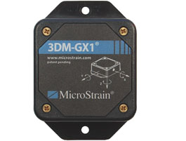
At a retail price of about $1495 US, it is one of the least expensive of industrial IMU devices (for comparison see http://www.xbow.com/Products/Inertial_Systems.htm) but still pretty pricey for most experimental roboticists. Several robot builders have been involved in developing less expensive versions. For example, see http://rotomotion.com as well as http://autopilot.sourceforge.net for some possible home-brew solutions. Several other manufacturers offer some combination of hardware and software solutions that might also be applicable, see for example:

http://www.o-navi.com
http://microboticsinc.com/ins_gps.php

A. 3DM-GX1 data

The 3DM-GX1 can return data in several formats depending on the commands sent to it by the controlling microprocessor.

1. Quaternion

   The "native" format returns data in a form known as a "quaternion" consisting of 4 floating point numbers, three of which comprise a 3-D vector and the forth represents a rotation around that vector to the sensors' current orientation. This is the most flexible format and does not suffer from the "singularities" that constrain the more common "Euler" format. However, it is somewhat more complex to decode.

2. Euler angles

   The sensor can also return data in a form more commonly used for navigation with the quantities Pitch, Roll, and Yaw, also know as Euler angles. (Conversion between quaternion and Euler angles is also possible on the main controlling microprocessor, at the expense of extra execution cycles). The 3DM-GX1 can perform the full measurement and conversion at a rate of about 50 Hz.

3. Raw sensor readings

   The 3DM-GX1 can also supply various raw and corrected sensor readings directly to the controlling microprocessor including magnetometer, accelerometer, and gyroscope data for further processing. These data sets can be arbitrarily mixed by issuing different commands to the device in sequence.

B. Euler angle command and data

The 3DM-GX1 Euler command (0x31) returns binary data over its serial port. The 0x31 command returns accelerations, rotations, a time stamp, and a checksum in addition to the Euler Pitch, Roll, and Yaw values.

The following "C" code defines a data structure that can be used by a micro-controller to receive the data from the 3DM-GX1 over a serial port:

	struct IMU {
        	short roll;		/* 16 bit signed Euler roll angle */
        	short pitch;		/* 16 bit signed Euler pitch angle */
        	unsigned short yaw;	/* 16 bit unsigned Euler yaw angle */
        	short accel_x;		/* 16 bit signed acceleration along the X axis */
        	short accel_y;		/* 16 bit signed acceleration along the Y axis */
        	short accel_z;		/* 16 bit signed acceleration along the Z axis */
        	short rate_x;		/* 16 bit signed rotation rate around X axis */
        	short rate_y;		/* 16 bit signed rotation rate around Y axis */
        	short rate_z;		/* 16 bit signed rotation rate around Z axis */
        	short ticks;		/* 16 bit 3DM-GX1 internal time stamp */
        	short chksum;		/* checksum */
	};

Roll and Pitch are signed values in which +- 90 degrees is represented by +- 32767. The Yaw value, which jBot uses for its theta heading number, is an unsigned 16 bit number which represents 0 through 2Pi radians (or 0 through 360 degrees) as 0 through 65535, where 0 represents magnetic north.

VI. jBot's 3DM-GX1 Implementation

JBot uses the 3DM-GX1 operating in its CONTINUOUS mode (0x10) which returns the EULER angle data (0x31) about 50 times per second in a free-running serial stream at 38400 baud.

A. IMU initialization

The following code sets up two of jBot's Motorola 68332 microprocessor TPU channels as a serial port and initializes the 3DM-GX1, using TPU system calls from the libmrm.a library as modified by Duane Gustavus and myself (not currently online), and initializes an interrupt routine named imu_int() to handle the data flow.

#define IMU_CMD 0x31
#define CONT_MODE 0x10

int imu_init(int chan, int baud)	/* channel number and baud rate */
{
        int extern vbraddr;

        imu_chan = chan;
        imu_baud = baud;
        
        /* init TPU channel as rx, channel+1 as tx, IMU uses 38400 baud */
        tpu_uart_init(imu_chan,1,imu_baud);              /* TPU chan, UART RX */
        tpu_uart_init(imu_chan+1,0,imu_baud);            /* TPU chan+1, UART TX */

        /* set CPU interrupt vector for TPU channel chan, (the receive interrupt) */
        *(long*)(vbraddr+(64*4)+(imu_chan*4)) = (long)imu_int;

        /* enable TPU interrupt for chan (receive interrupt) */
        tpu_set_cier(imu_chan,1);

        /* send the startup sequence to the IMU */
        while (tpu_send_char(imu_chan+1,CONT_MODE) == -1);      /* continuous mode */
        while (tpu_send_char(imu_chan+1,0x00) == -1);           /* terminate command */
        while (tpu_send_char(imu_chan+1,IMU_CMD) == -1);        /* Euler angles, rate, accel */

        return 0;
}

B. IMU interrupt

Data from the IMU is received by an interrupt routine running on the 68332 micro-controller which fills the imu input buffer structure, tests for a valid checksum, and updates the global "imu" structure if the data is valid, incrementing an error counter if not:

attribute__((__interrupt__)) void imu_int(void) 
{
        int byte;

	/* clear TPU interrupt flag for chan  */
        TPU_CISR &= ~(0x1 << imu_chan);    

	/* read the next input byte from TPU channel "imu_chan" */
        byte = (*(unsigned short *) (TPU_RAM + (imu_chan * 16 + 0x04)));

	/* test for valid IMU cmd */
        if (imu_state == 0) {
                if (byte == IMU_CMD) imu_state++;
        } else {
                *buf++ = (unsigned char)byte;
                imu_state++;
                if (imu_state == 23) {          /* 11 16bit words + command byte */
                        if (calc_checksum() == imu_buf.chksum) {
                                imu = imu_buf;  /* copy struct as 5 longs and 1 short, atomic */
                        } else {
                                imu_err++;
                        }
                        imu_state = 0;
                        buf = (unsigned char *)&imu_buf;	/* reset the buffer pointer */
                }
        }
}


int calc_checksum()
{
         imu_checksum = ((short)IMU_CMD + imu_buf.roll + imu_buf.pitch + imu_buf.yaw
                + imu_buf.accel_x + imu_buf.accel_y + imu_buf.accel_z
                + imu_buf.rate_x + imu_buf.rate_y + imu_buf.rate_z + imu_buf.ticks);

        return imu_checksum;
}

The end result of all of this is a global structure in memory on the 68332 micro-controller, updated about 50 times per second, that contains the Euler angles, accelerations, and rotations of the sensor, and hence the robot.

C. Physical placement

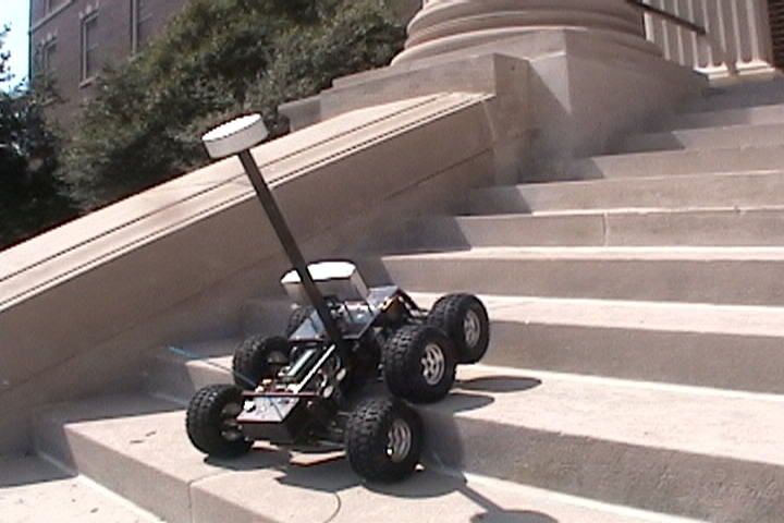
The magnetometers contained in the 3DM-GX1 can be calibrated using a routine internal to the device to account for local magnetic fields on the robot itself. However, they are apparently also influenced by the electrical fields of the robot's drive motors, which differ with the strength and direction of the motor currents. For this reason the sensor was eventually attached to the top of a mast about 2 feet tall, mounted in the center of the jBot platform, as can be seen in the following images, and in this image of jBot ascending a flight of stairs:

http://geology.heroy.smu.edu/~dpa-www/robo/jbot/jbot_steps_001.jpg

The sensor is mounted in a PVC housing attached to a carbon fiber tube which serves to protect and support it in the event that the robot flips upside down (it happens). This also serves to protect the expensive and non-standard little mil-spec serial connector that ships with the 3DM-GX1.

The height of the mast was determined empirically by running a series of 100 foot UMBmark tests in a large field, from several different points of the compass, until all tests produced approximately the same size errors.

VII. Integrating the 3DM-GX1 IMU with jBot's odometry

jBot is a 6-wheeled differentially steered robot with independent suspension and all-wheel drive. The basic odometry algorithm is identical to that used on SR04, with the exception that the WHEEL_BASE constant, determined experimentally using Borenstein's UMBmark, is the diagonal distance from the center of one front wheel to the center of the opposite rear wheel.

A. Traditional odometry

The first step is to implement and calibrate the standard encoder-driven odometry functions for jBot as describe above for the SR04 robot. Calibration of the odometry for a 6-wheel skid steered vehicle is problematic because the slippage of the fore and aft wheels as they "scrub" during rotation is highly dependent on the running surface. So the robot calibrated for a concrete surface behaves differently on grass and on gravel. jBot's odometry was calibrated on gravel as the best average fit between various surfaces. Note that this will also be true for a treaded vehicle such as a tank.

B. Integrating the IMU heading

Incorporating the heading from the 3DM-GX1 is simply a matter of reading the Yaw value from the imu struct maintained by the interrupt defined in section VI.B. above, scaling it appropriately, and substituting the value so obtained for the theta value normally calculated from the wheel encoders. The following "C" code implements this function along with a couple of other features that are described below.

/* ----------------------------------------------------------------------- */
/* robot geometry */

#define WHEEL_BASE 23.0         	/* corner-to-corner */
#define CLICKS_PER_INCH 4323.15         /* E-MAXX 5 inch wheels */
#define BIG_CLICKS_PER_INCH 3527.6	/* Rock-Crawler 7 inch wheels */

/* ----------------------------------------------------------------------- */
/* odometer maintains these global accumulator variables: */
/* ----------------------------------------------------------------------- */

float theta;            /* bot heading in radians minus theta_offset */
float theta_global;     /* global theta from IMU, radians */
float theta_offset;     /* offset from from global theta to local theta */
float X_pos;            /* bot X position in inches */
float Y_pos;            /* bot Y position in inches */

/* rate of rotation measurements, used for stasis error detection */

float wheel_theta;      /* change in theta calculated from wheels */
float imu_theta;        /* change in theta calculate from IMU */

/* ----------------------------------------------------------------------- */
/* local variables */

float left_inches;
float right_inches;
float avg_inches;
float clicks_per_inch;
float last_theta;      

/* ----------------------------------------------------------------------- */

void odometers()
{
        extern int stasis();
        extern struct IMU imu;
        extern int left_velocity, right_velocity;
        int t;

        if (g->wheelsize == 1) {
                clicks_per_inch = BIG_CLICKS_PER_INCH;
        } else {
                clicks_per_inch = CLICKS_PER_INCH;
        }

        t = mseconds();
        while (1) {

                left_inches = (float)(left_velocity) / clicks_per_inch;
                right_inches = (float)(right_velocity) / clicks_per_inch;

                avg_inches = (left_inches + right_inches) / 2.0;
                total_inches += avg_inches;

                wheel_theta = (left_inches - right_inches) / WHEEL_BASE;

		/* read the YAW value from the imu struct and convert to radians */
                theta_global = ((float)imu.yaw*TWOPI)/65536.0;

		/* calculate rotation rate-of-change for stasis detector */
                imu_theta = theta_global - last_theta;
                last_theta = theta_global;

                if (g->yaw_enable) {
                        theta  = theta_global;
                } else {
                        theta += wheel_theta;
                }

                theta -= (float)((int)(theta/TWOPI))*TWOPI;
                if (theta < -PI) { theta += TWOPI; }
                else { if (theta > PI) theta -= TWOPI; }

                X_pos += (float)(avg_inches * sin(theta)); 
                Y_pos += (float)(avg_inches * cos(theta)); 

                stasis(fabs(wheel_theta),fabs(imu_theta));

            t = tsleep(t,50);
        }
}

The routine actually calculates two theta values, one from the wheel encoders and one from the IMU. If the global flag (g->yaw_enabled) is set, the robot uses the IMU's theta (the normal case) otherwise it uses the theta derived from the wheel encoders. This allows the robot to fall back on the wheel odometry if it loses the IMU signal. So far that's never happened.

A couple of steps are left out of this algorithm for clarity. One is an offset which allows the global theta to be rotated into the coordinate system of the robot, rather than using a coordinate system based on true north. This is handy if, for example, you would like the robot to go "straight ahead" for some distance, irrespective of the actual direction of North. The other is a correction based on the local magnetic variation from true north, as derived from the robot's GPS unit, which allows the robot to seek accurately on GPS and map coordinates. Finally, the routine "stasis()" is used to determine when the robot is stuck, as described below in section IX.

VIII. jBot's IMU-corrected Odometry performance

The combination of wheel odometry with the 3DM-GX1 orientation sensor gives jBot the ability to track its location across uneven terrain with an accuracy of less than +-.5% of distance traveled.

A. Performance over uneven terrain

Here is a 5 Meg mpeg movie of jBot running a simple program that seeks to go repeatedly between two coordinates 20 feet apart, (0,240)(0,0) using the IMU's measurement of theta. This is a good quick test for determining drift in the location calculations.

This particular run over an uneven surface checks the ability of the IMU to maintain a heading when not level. Note that the IMU in these tests was mounted on a wooden dowel, and the robot had not yet acquired its SONAR array:

http://www.geology.smu.edu/~dpa-www/robo/jbot/jbot_rough_01.mp4

B. Performance while avoiding obstacles

Here is a 21 Meg mpeg movie of jBot attempting to navigate to a point 500 feet away and back, (0,6000)(0,0) while using its SONAR array to avoid obstacles such as trees and picnic tables along the way. For a total journey of over 1000 feet, the errors are typically +- 5 feet at the end. However, an error of +- 5 feet means that SOMETIMES, randomly, the error is very close to 0, as in this case. The robot returns almost exactly to its starting place, as marked by a straw hat dropped at the origin (hence the video name "hat trick"):

http://www.geology.smu.edu/~dpa-www/robo/jbot/jbot_hatrick2_2.mp4

I ran this test 4 more times and each time the robot arrived within about 5 feet of the hat, but I have not as of this writing been able to get it again to hit the hat directly.

IX. Other conditions measured by the IMU

The 3DM-GX1 Euler command returns several other numbers that are useful for determining the robot's status, including the PITCH and ROLL values. Accelerations, currently not used, might also be valuable to detect collisions, slow the robot down on particularly rough terrain, and perhaps even be integrated to velocities in order to provide a check on wheel slippage and sideways motion. Currently jBot uses its GPS measured coordinates to detect and correct gross odometry errors caused by wheel slippage, on the order of a dozen feet.

A. Pitch and Roll

The IMU values Pitch (nose up and down) and Roll (tilt left and right) are used in a separate routine by jBot to detect when the robot is approaching dangerously steep angles. In the current code, a robot escape() routine is triggered when the platform exceeds 60 degrees from horizontal in any direction. This same escape() routine is also triggered when the robot determines that its wheels are stuck and unable to rotate. The escape() behavior attempts to back up, wiggle left or right, drive forward, and so forth until the trigger condition is no longer met.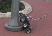

Here is a 5.8 Meg mpeg video of jBot climbing a pole during the development of the SONAR obstacle detection array, triggering the escape() behavior as the IMU Pitch value exceeds 60 degrees.

http://www.geology.smu.edu/~dpa-www/robo/jbot/jbot2/jbot_tilt.mp4

B. Stasis

The imu_theta variable calculated in jBot's odometry() routine is a rate-of-change value, the first derivative of the robot's rotation around the Z axis, that is used to detect when the robot is stuck but it's wheels are still turning. This works because the robot, when trapped, is invariably trying to rotate to get itself free.

The basic premise is fairly simple. The rate of rotation measured by the IMU and that calculated from the wheel encoders should normally be about the same, irrespective of how the two may drift apart in actual heading determination.

When the two are very different, particularly when the wheel encoders report that the robot is rotating and the IMU reports that it is not, the robot is probably stuck.

So by calculating a running difference between the two rate-of-rotation values, the robot can know that it is stuck and take appropriate steps to get free. The stasis() routine is called with the two rate-of-rotation values as the last step in the odometry() routine. The "C" code looks like this:

/* ----------------------------------------------------------------------- */
/* stasis detector      */
/* ----------------------------------------------------------------------- */

#define NOT_TURNING .005
#define ARE_TURNING .010
#define STASIS_ERR 60

/* stasis detector globals */

int stasis_err;         /* number of times imu and wheels very different */
int stasis_alarm;       /* signal too many stasis errors */
                        /* this is read by escape() in escape.c */

/* ----------------------------------------------------------------------- */

int stasis(wheel_drv, imu_drv)
float wheel_drv, imu_drv;
{

        if ((imu_drv < NOT_TURNING) && (wheel_drv > ARE_TURNING)) { 
                stasis_err++;
        } else {
                if (stasis_err) stasis_err--;
                else stasis_alarm = 0;
        }
                
        if (stasis_err > g->stasis_err) {
                stasis_alarm = 1;
                stasis_err = 0;
        } 

        return 0;
}

/* ----------------------------------------------------------------------- */

The variable stasis_err is incremented whenever stasis conditions are met and decremented to 0 when they are not met. This integration acts as a simple low pass filter that prevents the escape() behavior from triggering too often, as when the robot is stuck only momentarily and then wiggles free, but also insures a trigger when the robot is bouncing around such that sometimes the wheel theta and IMU theta agree, but the robot actually is trapped. When the stasis_err exceeds a global limit set by the user, the escape alarm is triggered. That limit is currently set such that the robot normally has about 2 seconds to free itself before the alarm is activated.

D. Stasis detection performance

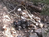
The following 16 Meg mpeg video is a composite made in the Colorado Rockies of several situations in which jBot found itself trapped and triggered a series of escape() behaviors in order to free itself. In each case, the robot was seeking on a distant coordinate while attempting to steer around obstacles, trees, miscellaneous forest detritus, and the Rocky Mountains in general.

http://geology.heroy.smu.edu/~dpa-www/robo/jbot/jbot2/jbot_unstuck.mp4

In the first section the robot collides with an unseen utility pole guy-wire and attempts to turn away for about two seconds before the stasis() alarm triggers. Thereafter a simple backup-and-turn collision recovery behavior serves to free the robot but leaves it pointing away from the target waypoint, such that the odometry-driven navigation must then re-acquire the proper heading.

The last section, in which the robot becomes high-centered on a fallen tree limb, exercises all of the robot's set of escape behaviors in sequence as it attempts to get free and finally continue its journey.

X. Conclusions

The Orientation sensor and Odometry combination provides a robust navigation system for an outdoor mobile robot, without the need of external reference signals, beacons, or visual markers. The main downside of this approach appears to be the cost, which is substantial when compared with most experimental robot sensors (though cheap by comparison to industrial IMUs or the ever-popular SICK laser scanners). However, recent advances by various researchers and manufacturers suggest that this cost might come down markedly in the not-too-distance future.

In addition to the use as a navigation aid, the IMU is also useful for detection and recovery from certain critical angles and trapped conditions of the robot.

I also believe that I can probably get jBot to balance on two wheels, like the balancing nBot robot, using this IMU. That might add considerable stability to the platform, prevent it from flipping over back-wards on steep inclines, and be generally amazing and entertaining for the local human population as well.

Special thanks to Ed Paradis of the DPRG for preparing the HTML formating and markup of this article.

dpa
10 October 2006
Dallas, Texas